神经网络解决非线性回归问题，调整层数，激活函数等未取得好的效果，求各位大神指导

Question

1.利用神经网络去解决多维非线性回归问题遇到问题
2.代码如下

# --------------------------------------------------------------------------------------------------------------模块导入
import time
import matplotlib.pyplot as plt
import DNCR.two_dimension.v3_NN.get_data as get_data
import tensorflow as tf
import numpy as np
import DNCR.two_dimension.v3_NN.Normalize_data as Normalize
# ----------------------------------------------------------------------------------------------------------------------

# ----------------------------------------------------------------------------------------------------------获取开始时间
start = time.process_time()
# ----------------------------------------------------------------------------------------------------------------------

# --------------------------------------------------------------------------------------------------训练数据和待预测数据
#  获得归一化特征数据集
feature_train, feature_new = Normalize.normalize_feature(get_data.get_kn_feature(['Kn30-J-feature.dat', 
                                                                                  'Kn30-J-feature.dat']), 1, 1)
# 获得归一化标记数据集及每个标记值的数值大小跨度
sign_train, max_min_len = Normalize.normalize_sign(get_data.get_delta_sign(['Kn30-J-sign.dat']))
sign_new = get_data.get_delta_sign(['Kn30-J-sign.dat'])
# ----------------------------------------------------------------------------------------------------------------------

# ----------------------------------------------------------------------------------------------------------------------
# 定义placeholder
x = tf.placeholder(tf.float32, [None, 5])  # 行不确定，有5列
y = tf.placeholder(tf.float32, [None, 1])  # 每个标记值训练一个神经网络
# ----------------------------------------------------------------------------------------------------------------------


# ----------------------------------------------------------------------------------------------------------神经网络函数
def neural_func():
    Weights_L1 = tf.Variable(tf.random_normal([5, 40]))  # 5行40列
    biases_L1 = tf.Variable(tf.zeros([1, 40]))  # biase永远为1行，列数和权重列数保持一致
    Wx_plus_b_L1 = tf.matmul(x, Weights_L1) + biases_L1
    L1 = tf.nn.sigmoid(Wx_plus_b_L1)

    Weights_L2 = tf.Variable(tf.random_normal([40, 80]))  
    biases_L2 = tf.Variable(tf.zeros([1, 80]))  
    Wx_plus_b_L2 = tf.matmul(L1, Weights_L2) + biases_L2
    L2 = tf.nn.sigmoid(Wx_plus_b_L2)

    Weights_L3 = tf.Variable(tf.random_normal([80, 40]))  
    biases_L3 = tf.Variable(tf.zeros([1, 40])) 
    Wx_plus_b_L3 = tf.matmul(L2, Weights_L3) + biases_L3
    L3 = tf.nn.sigmoid(Wx_plus_b_L3)

    Weights_L4 = tf.Variable(tf.random_normal([40, 20]))
    biases_L4 = tf.Variable(tf.zeros([1, 20]))
    Wx_plus_b_L4 = tf.matmul(L3, Weights_L4) + biases_L4
    L4 = tf.nn.sigmoid(Wx_plus_b_L4)

    # Weights_L5 = tf.Variable(tf.random_normal([20, 100]))
    # biases_L5 = tf.Variable(tf.zeros([1, 100]))
    # Wx_plus_b_L5 = tf.matmul(L4, Weights_L5) + biases_L5
    # L5 = tf.nn.tanh(Wx_plus_b_L5)
    #
    # Weights_L6 = tf.Variable(tf.random_normal([100, 100]))
    # biases_L6 = tf.Variable(tf.zeros([1, 100]))
    # Wx_plus_b_L6 = tf.matmul(L5, Weights_L6) + biases_L6
    # L6 = tf.nn.tanh(Wx_plus_b_L6)
    # ------------------------------------------------------------------------------------------------------------------

    # ------------------------------------------------------------------------------------------------------------输出层
    Weights_L7 = tf.Variable(tf.random_normal([20, 1]))
    biases_L7 = tf.Variable(tf.zeros([1, 1]))
    Wx_plus_b_L7 = tf.matmul(L4, Weights_L7) + biases_L7
    prediction = tf.nn.tanh(Wx_plus_b_L7)
    return prediction
# ----------------------------------------------------------------------------------------------------------------------


# ----------------------------------------------------------------------------------------------------------神经网络训练
prediction = neural_func()
loss = tf.reduce_mean(tf.square(y - prediction))  # 损失函数
train_step = tf.train.GradientDescentOptimizer(0.05).minimize(loss)  # 使用梯度下降法训练
result = []  # 结果列表
with tf.Session() as sess:
    for i in range(len(sign_train)):
        sess.run(tf.global_variables_initializer())  # 变量初始化
        for _ in range(10000):
            sess.run(train_step, feed_dict={x: feature_train, y: np.transpose(sign_train[i])})  # 训练
            print(sess.run(loss, feed_dict={x: feature_train, y: np.transpose(sign_train[i])}))  # 输出每步损失值
        prediction_value = sess.run(prediction, feed_dict={x: feature_new})  # 获得预测值
        result.append(np.transpose(prediction_value*max_min_len[i]).tolist()[0])
# ----------------------------------------------------------------------------------------------------------------------

# ----------------------------------------------------------------------------------------------------------------可视化
title_list = ['Delta(hfx)', 'Delta(hfy)', 'Delta(tauxx)', 'Delta(tauxy)', 'Delta(tauyy)',  'Delta(RuRx)',
              'Delta(RvRx)', 'Delta(RTRx)', 'Delta(RuRy)',  'Delta(RvRy)',  'Delta(RTRy)']  # 图标题列表


def Visual_func():
    for i in range(len(result)):
        title = title_list[i]
        plt.title(title, fontsize='xx-large')
        plt.plot(range(len(result[i])), sign_new[i], c='y', marker='o')
        plt.plot(range(len(result[i])), result[i], c='b', marker='*')
        # 设置刻度字体大小
        plt.xticks(fontsize=20)
        plt.yticks(fontsize=20)
        plt.legend(['Train-I', 'Predict-I'], fontsize=20, loc='best')
        plt.show()


Visual_func()
time_length = time.process_time() - start
print('运行结束!程序运行时间为:', time_length, 's')

输入与输出也进行了归一化，输出也进行了反归一化，效果一直不好。

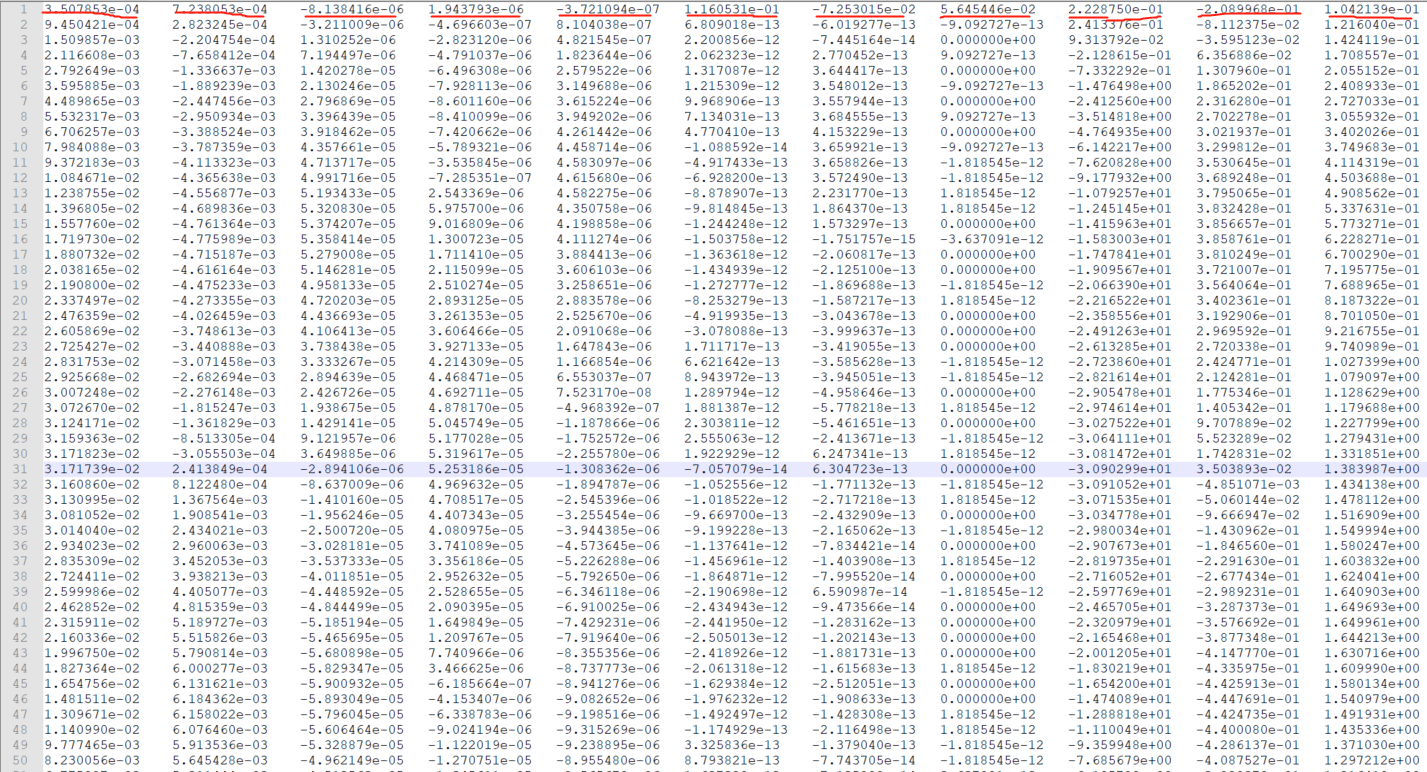
如下图所示，第一张图片中每行代表一个样本，第二张图片中每行中的单个数据代表需要得到的非线性回归关系，总共11个关系。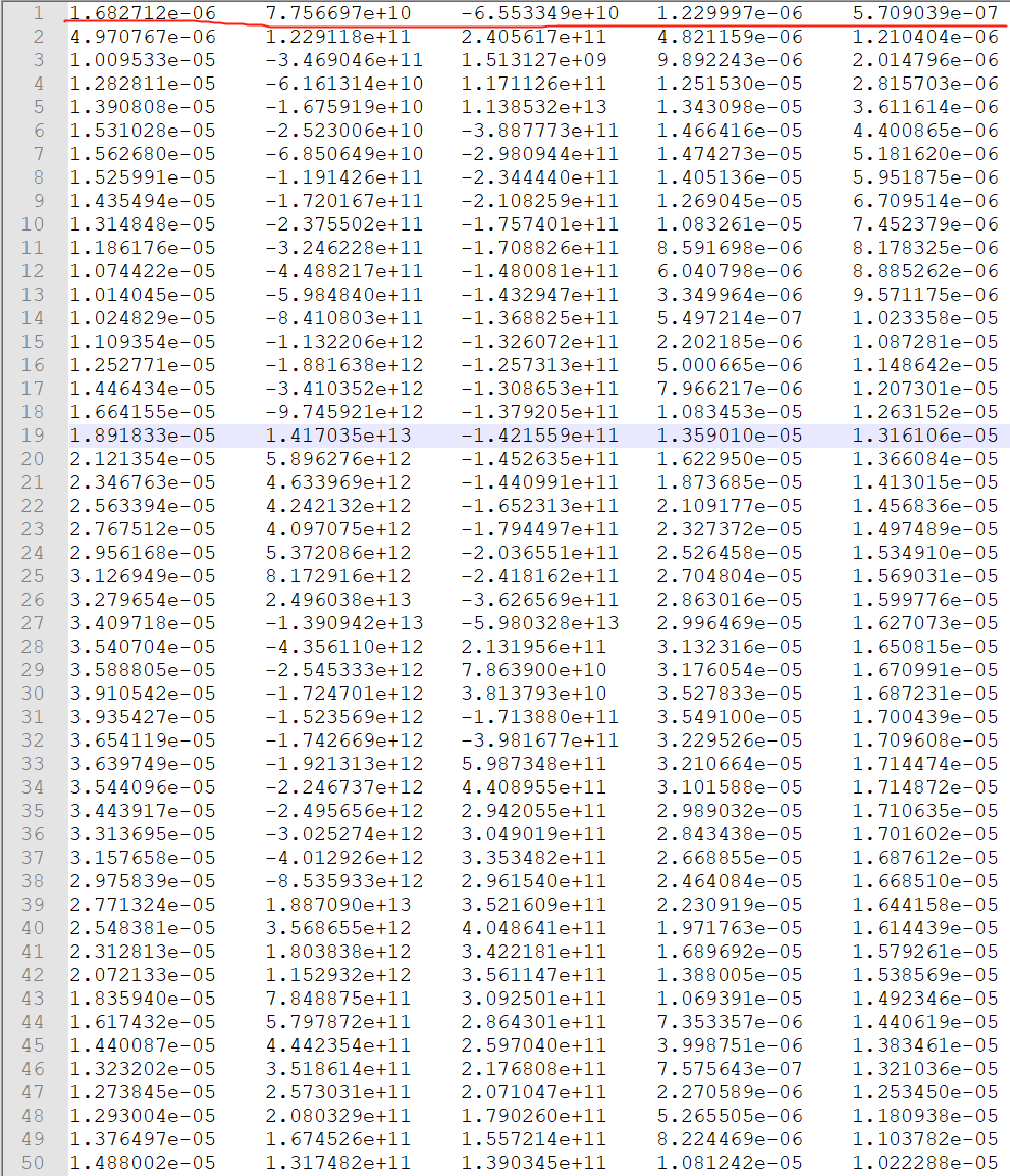


如果有大佬能帮忙解决，感激不尽。
(导入的模块中有两个自编模块)以及数据还未上传，可以联系找我要。

Answer 1

https://blog.csdn.net/qq_27261889/article/details/85015013