
使用python curve_fit 拟合函数如图
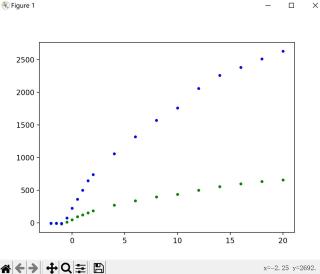
根据查阅资料,光电效应的伏安特性曲线拟合形式大致时y=k(ax+b)^0.5的形式
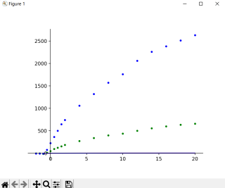
但是拟合结果如图
我写的核心代码如下
#使用curve_fit做给定函数形式的拟合
#引入模块scipy.optimize 的curve_fit
from scipy.optimize import curve_fit as c_fit
#首先定义拟合函数
def func(x,k,a,b):
    return k*np.power(a*x+b,0.5)
x3=np.array(x3)
y3_1=np.array(y3_1)
y3_2=np.array(y3_2)
###利用拟合函数求特征值##
popt1,pcov1 = c_fit(func,x3,y3_1,bounds=([-np.inf,-np.inf,-np.inf],[np.inf,np.inf,np.inf]),maxfev = 10000)
popt2,pcov2 = c_fit(func,x3,y3_2,bounds=([-np.inf,-np.inf,-np.inf],[np.inf,np.inf,np.inf]),maxfev = 10000)

###R^2最小二乘计算###
calc_y1 = [func(i, popt1[0], popt1[1],popt1[2]) for i in x3]
res_y1 = np.array(y3_1) - np.array(calc_y1)
ss_res1 = np.sum(res_y1 ** 2)
ss_tot1 = np.sum((y3_1 - np.mean(y3_1)) ** 2)
r_squared1 = 1 - (ss_res1 / ss_tot1)

calc_y2 = [func(i, popt2[0], popt2[1],popt2[2]) for i in x3]
res_y2 = np.array(y3_2) - np.array(calc_y2)
ss_res2 = np.sum(res_y2 ** 2)
ss_tot2 = np.sum((y3_2 - np.mean(y3_2)) ** 2)
r_squared2 = 1 - (ss_res2 / ss_tot2)

###拟合的结果###
y3n1 = [func(i,popt1[0],popt1[1],popt1[2]) for i in x3]
y3n2 = [func(i,popt2[0],popt2[1],popt2[2]) for i in x3]
print(popt1)
print(popt2)
print("k = %f  a = %f   b = %f r=%f" % (popt1[0], popt1[1],popt1[2], r_squared1))
print("k = %f  a = %f   b = %f r=%f" % (popt2[0], popt2[1],popt2[2], r_squared2))
ax=py.gca()#获取边框位置
ax.spines['right'].set_color('none')
ax.spines['top'].set_color('none')#取消上右边框
ax.spines['bottom'].set_position(('data',0))#将x轴绑定在y=0处,data表示将绑定到轴处
ax.spines['left'].set_position(('data',0))#将y轴绑定在x=0处
###绘图###
py.plot(x3,y3n1,'r-')
py.plot(x3,y3n2,'b-')
py.show()
其中excel数据

光阑\电压: -2 -1.50 -1 -0.50 0 0.50 1 1.50 2 4 6 8 10 12 14 16 18 20
2mm时的电流 -2.10 -1.70 -13 15.50 50.50 95 125 156 185 275 340 400 440 500 558 601 636 660
4mm时的电流 -7.40 -7.30 -5.30 76 225 364 500 645 740 1,060 1,320 1,570 1,760 2,060 2,260 2,380 2,510 2,630


