
请根据图片,分析一下我这个自适应光学系统是否搭建成功?
```bash
clc
clear
close all
%%参数设置
z = 3000; % 传输距离 (单位: 米)
N = 256; % 采样点数目
w0 = 0.1; % 束腰半径 (单位: 米)
Cn2 = 1e-15; % 湍流结构常数
lambda = 1550*10.^-9; % 波长 (单位: 米)
L = 1; % 输入屏尺寸 (单位: 米)
L2 = 1; % 相位屏尺寸 (单位: 米)
bushu = 25; % 相位屏数量
noise_level = 0.1; % 噪声水平调节因子
N_sub = 16; % 每个微透镜对应的子孔径像素数
f_lens = 0.04; % 微透镜焦距 (单位: 米)
% 子孔径掩膜
[x, y] = meshgrid(1:N_sub, 1:N_sub);
center = (N_sub + 1) / 2;
r = sqrt((x - center).^2 + (y - center).^2);
radius = N_sub / 2;
aperture_mask = double(r <= radius);
num_modes = 36; % 使用的 Zernike 模式数
nLayers = 6; % 示例促动器层数
sigma = 1.5; % 示例高斯函数标准差
pitch = 0.05; % 示例促动器间距
mirrorSize = [120, 120]; % 示例变形镜尺寸
% SPGD算法参数
step_size = 0.05; % 步长
max_iterations = 200; % 最大迭代次数
decay = 0.98;
min_step_size = 0.01;
% 初始生成大气湍流相位屏和光场
[I0, I1, I3, UT, phase3] = generate_von_karman_phase_screen(z, N, w0, Cn2, lambda, L, L2, bushu, noise_level);
[slope_x, slope_y] = shack_hartmann_measurement(I1, I3, N_sub, L,N, f_lens,aperture_mask);
[phase_reconstruction, G,Z_coeff] = zernike_wavefront_reconstruction(N, L, N_sub, slope_x, slope_y, num_modes,aperture_mask);
[B,V]=control(slope_x,slope_y,G,num_modes,nLayers,sigma,pitch,mirrorSize);
[corrected_I,phase_corrected] = correction( phase_reconstruction,UT,V,mirrorSize,nLayers, pitch,sigma);
[actuator_pos, num_Actuators] = generateHexActuators(nLayers, pitch);
% SPGD算法迭代
for iteration = 1:max_iterations
% 计算性能指标
strehl_ratio = calculate_strehl_ratio(I1, phase_corrected);
rmse = calculate_rmse(phase3, phase_corrected);
% 检查是否满足条
if strehl_ratio > 0.905 && rmse < 1.65
disp('优化目标已达到,停止迭代。');
break;
end
% 生成随机扰动
delta_V = randn(num_Actuators, 1);
% 正向扰动
V_plus = V + step_size * delta_V;
[corrected_I_plus,phase_corrected_plus] = correction( phase_reconstruction,UT,V_plus,mirrorSize,nLayers, pitch,sigma);
strehl_ratio_plus = calculate_strehl_ratio(I1, corrected_I_plus);
rmse_plus = calculate_rmse(phase3, phase_corrected_plus);
% 负向扰动
V_minus = V - step_size * delta_V;
[corrected_I_minus,phase_corrected_minus] = correction( phase_reconstruction,UT,V_minus,mirrorSize,nLayers, pitch,sigma);
strehl_ratio_minus = calculate_strehl_ratio(I1, corrected_I_minus);
rmse_minus = calculate_rmse(phase3, phase_corrected_minus);
% 计算梯度
gradient_strehl = (strehl_ratio_plus - strehl_ratio_minus) / (2 * step_size);
gradient_rmse = (rmse_plus - rmse_minus) / (2 * step_size);
% 综合目标函数的权重
alpha = 0.5; % Strehl 比的权重
beta = 0.5; % RMSE 的权重
% 更新系数矩阵
V = V + step_size * (alpha * gradient_strehl - beta * gradient_rmse);
[corrected_I,phase_corrected] = correction( phase_reconstruction,UT,V,mirrorSize,nLayers, pitch,sigma);
% 显示当前迭代结果
disp(['Iteration ', num2str(iteration), ': RMSE = ', num2str(rmse), ', Strehl Ratio = ', num2str(strehl_ratio)]);
% 步长更新策略
% 1. 基于迭代次数的衰减
if mod(iteration, 10) == 0
step_size = max(step_size * decay, min_step_size);
end
% 检查是否达到最大迭代次数
if iteration >= max_iterations
disp('达到最大迭代次数,停止优化。');
break;
end
end
visualize_results(I0, I1, I3, corrected_I, phase3,phase_reconstruction, phase_corrected, strehl_ratio, rmse);
function[I0, I1, I3, UT, phase3] = generate_von_karman_phase_screen(z, N, w0, Cn2, lambda, L, L2, bushu, noise_level)
% 计算基本参数
k = 2 * pi / lambda; % 波数
delta = L / N; % 空间采样间隔
x = (-N/2:N/2-1) * delta;
y = x;
[X, Y] = meshgrid(x, y);
[~, r] = cart2pol(X, Y);
% 高斯光束参数
z1 = 0; % 束腰位置
n_i = 1.0; % 背景空间折射率
k0 = k * n_i; % 背景空间的波数
ZR = k0 * w0^2 / 2; % 瑞利距离
w = w0 * sqrt(1 + (z1 / ZR)^2); % 传播到 z1 处的束宽
R = ZR * (z1 / ZR + ZR / z1); % 等相位面曲率半径
Phi = atan(z1 / ZR); % 相位因子
% 高斯光束电场表达式
E0 = (1 / (1 + 1i * z1 / ZR)) .* exp(-(r.^2 / w0^2) ./ (1 + 1i * z1 / ZR)) .* exp(1i * k0 * z1);
% 源场光场
I0 = abs(E0).^2;
% 未加湍流条件下的传输
x1 = linspace(-L / 2, L / 2, N).*N; % 频域坐标
y1 = linspace(-L / 2, L / 2, N).*N;
[kethi, nenta] = meshgrid(x1, y1);
U0 = E0;
H = exp(1i * k * z * (1 - (lambda^2) * (kethi.^2 + nenta.^2) / 2)); % 传递函数
G0 = fftshift(fft2(U0)); % 衍射面上光场的傅里叶变换
G = G0 .* H; % 光场的频谱与传递函数相乘
U = ifft2(G); % 在观察屏上的光场分布
I1 = U .* conj(U); % 在观察屏上的光强分布
% 加湍流条件下的传输
deltz = z / bushu; % 相位屏间距
l0 = 0.01; % 内尺度
L0 = 10; % 外尺度
r0 = (0.4229 * (k^2) * Cn2 * deltz)^(-3/5); % 大气相干长度
subh = 8; % 次谐波次数
delta1 = L2 / N; % 相位屏采样间隔
fx = (-N/2:N/2-1) * (1 / (N * delta1)); % 横向频率
[kx, ky] = meshgrid(2 * pi * fx); % 生成网格坐标矩阵
[~, ka] = cart2pol(kx, ky); % 转换为极坐标
km = 5.92 / l0; % 内尺度对应的波数
k0 = 2 * pi / L0; % 外尺度对应的波数
PSD_phi = 0.033 * Cn2 * exp(-(ka / km).^2) ./ (ka.^2 + k0.^2).^(11/6); % 冯卡门谱
PSD_phi(N/2+1, N/2+1) = 0; % 避免除以零
cn = 2 * pi * (k^2) * deltz * PSD_phi * (2 * pi * (1 / (N * delta1)))^2; % 相位扰动的幅度
UT = E0;
for l = 1:bushu
% 生成高频相位屏
phz_hi = ift2(noise_level * (randn(N) + 1i * randn(N)) .* sqrt(cn), 1);
phz_hi = real(phz_hi);
% 低频补偿
phz_lo = zeros(size(phz_hi));
for p = 1:subh
del_fp = 1 / (3^p * L2);
fx1 = (-1:1) * del_fp;
[kx1, ky1] = meshgrid(2 * pi * fx1);
[th1, k1] = cart2pol(kx1, ky1);
PSD_phi1 = 0.033 * Cn2 * exp(-(k1 / km).^2) ./ (k1.^2 + k0.^2).^(11/6);
PSD_phi1(2, 2) = 0;
cn1 = 2 * pi * k^2 * deltz * PSD_phi1 * (2 * pi * del_fp)^2;
cn1 = noise_level * (randn(3) + 1i * randn(3)) .* sqrt(cn1);
SH = zeros(N);
for ii = 1:9
SH = SH + cn1(ii) * exp(1i * (kx1(ii) * X + ky1(ii) * Y));
end
phz_lo = phz_lo + SH;
end
phz_lo = real(phz_lo) - mean(real(phz_lo(:)));
phz = phz_hi + phz_lo;
figure (5)
pcolor(kx,ky,phz);
colormap("jet")
axis on;
shading interp;
axis square; %输出正方形图像
colorbar;
title("低频补偿后的大气湍流随机相位屏");
% 判断是否是第一次循环,第一次循环时不叠加随机相位屏
if l == 1
G1 = fftshift(fft2(UT));
else
UT = UT .* exp(1i * phz);
G1 = fftshift(fft2(UT));
end
% 光场传播
x2 = linspace(-L/2, L/2, N) * N;
y2 = linspace(-L/2, L/2, N) * N;
[kethi2, nenta2] = meshgrid(x2, y2);
H = exp(1i * k * deltz * (1 - (lambda^2)*(kethi2.^2 + nenta2.^2)/2));
G1 = G1 .* H;
UT = ifft2(G1);
% 可视化中间结果(可选)
if l ~= bushu
I2 = UT .* conj(UT);
figure(3);
pcolor(x, y, I2);
nu = l-1;
title("经"+nu+"次大气湍流传输后的光场");
colormap("jet");
colorbar;
axis on;
shading interp;
axis square; %输出正方形图像
axis image;
xlabel('{\itx}(m)');
ylabel('{\ity}(m)');
end
end
% 最终光强分布
I3 = UT .* conj(UT);
phase3 = angle(UT) ;
end
function g = ift2(G, delta_f)
% function g = ift2(G, delta_f)
N = size(G, 1);
g = ifftshift(ifft2(ifftshift(G)))*(N*delta_f)^2;
end
function [slope_x, slope_y] = shack_hartmann_measurement(I1, I3, N_sub, L, N, f_lens, aperture_mask)
% 获取光强分布的尺寸
[N, ~] = size(I1);
% 计算子孔径的数量
num_sub_x = floor(N / N_sub);
num_sub_y = floor(N / N_sub);
% 初始化质心偏移量矩阵
centroid_offset_x = zeros(num_sub_y, num_sub_x);
centroid_offset_y = zeros(num_sub_y, num_sub_x);
% 遍历每个子孔径计算质心偏移
for i = 1:num_sub_y
for j = 1:num_sub_x
% 提取当前子孔径的光强分布
start_row = (i - 1) * N_sub + 1;
end_row = start_row + N_sub - 1;
start_col = (j - 1) * N_sub + 1;
end_col = start_col + N_sub - 1;
% 应用孔径掩码
sub_I1 = I1(start_row:end_row, start_col:end_col) .* aperture_mask;
sub_I3 = I3(start_row:end_row, start_col:end_col) .* aperture_mask;
% 计算质心并转换为物理单位
[centroid_x1, centroid_y1] = calculate_centroid(sub_I1);
[centroid_x3, centroid_y3] = calculate_centroid(sub_I3);
centroid_offset_x(i, j) = (centroid_x3 - centroid_x1) * (L/N);
centroid_offset_y(i, j) = (centroid_y3 - centroid_y1) * (L/N);
end
end
% 计算波前斜率
slope_x = centroid_offset_x/ f_lens;
slope_y = centroid_offset_y / f_lens;
end
function [centroid_x, centroid_y] = calculate_centroid(I)
% 计算光斑质心
[rows, cols] = size(I);
[X, Y] = meshgrid(1:cols, 1:rows);
total_intensity = sum(I(:));
centroid_x = sum(sum(I .* X)) / total_intensity;
centroid_y = sum(sum(I .* Y)) / total_intensity;
end
function [phase_reconstruction, G,Z_coeff] = zernike_wavefront_reconstruction(N, L, N_sub, slope_x, slope_y, num_modes,aperture_mask)
del=L/N;
x1 = (-N/2: N/2-1)*del ;
y1=x1;
%生成全局坐标系
[X, Y] = meshgrid(x1,y1);
rho = sqrt((X).^2 + (Y ).^2)/sqrt((L/2)^2 + (L/2)^2);
theta = atan2(Y , X );
%生成子孔径坐标系
x2= (-N_sub/2:N_sub/2-1)*del;
y2=x2;
[X_sub, Y_sub] = meshgrid(x2, y2);
rho12 = sqrt((X_sub).^2 + (Y_sub).^2)/sqrt((N_sub*del/2)^2 + (N_sub*del/2)^2);
theta12 = atan2(Y_sub , X_sub );
% 生成Noll顺序的Zernike模式索引
modes = generate_noll_modes(num_modes);
% 获取子孔径数量并初始化G矩阵
num_sub_x = floor(N / N_sub);
num_sub_y = floor(N / N_sub);
K = num_sub_y * num_sub_x;
G = zeros(2*K, num_modes);
% 构建G矩阵
for i = 1:num_sub_y
for j = 1:num_sub_x
k = (i-1)*num_sub_x + j;
s_sub_x = L / num_sub_x; % 子孔径物理宽度
s_sub_y = L / num_sub_y; % 子孔径物理高度
z = s_sub_x*s_sub_y;
for m_idx = 1:num_modes
n = modes(m_idx, 1);
m = modes(m_idx, 2);
Z = zernike_poly(n, m, rho12, theta12);
dZdx = gradient(Z, del, 1); % x方向梯度(列方向)
dZdy = gradient(Z, del, 2); % y方向梯度(行方向)
dx = s_sub_x/N_sub;
dy = s_sub_y/N_sub;
F_x=(sum(sum(dZdx .* aperture_mask) )* dx * dy)/z;
F_y=(sum(sum(dZdy .* aperture_mask) )* dx * dy)/z;
G(2*k-1, m_idx) =F_x;
G(2*k, m_idx) =F_y;
end
end
end
%disp(G);
%disp(Z);
% 构建斜率向量并求解系数
s = [slope_x(:); slope_y(:)];
alpha = 1e-4; % 正则化参数
Z_coeff = (G'*G + alpha*eye(num_modes)) \ (G'*s);
% 生成Noll模式
modes = generate_noll_modes(num_modes);
% 初始化相位畸变
phase_reconstruction = zeros(size(X));
% 计算Zernike多项式叠加
for m_idx = 1:num_modes
n = modes(m_idx, 1);
m = modes(m_idx, 2);
Z = zernike_poly(n, m, rho, theta);
phase_reconstruction = phase_reconstruction + Z_coeff(m_idx) * Z;
end
end
function modes = generate_noll_modes(M)
modes = zeros(M, 2);
idx = 1;
n = 0;
while idx <= M
m_candidates = -n:2:n;
valid_m = m_candidates(mod(n + abs(m_candidates), 2) == 0);
valid_m = unique(valid_m);
positive_m = valid_m(valid_m > 0);
zero_m = valid_m(valid_m == 0);
negative_m = valid_m(valid_m < 0);
sorted_m = [];
if ~isempty(positive_m)
sorted_m = [sort(positive_m, 'descend')]; % 正m降序
end
if ~isempty(zero_m)
sorted_m = [sorted_m, 0];
end
if ~isempty(negative_m)
sorted_m = [sorted_m, sort(negative_m, 'descend')]; % 负m降序(绝对值升序)
end
for i = 1:length(sorted_m)
if idx > M
break;
end
modes(idx, :) = [n, sorted_m(i)];
idx = idx + 1;
end
n = n + 1;
end
end
function Rnm = radial_polynomial(n, m, rho)
% 验证输入参数,确保n - m为偶数,否则返回全零数组
if mod(n - m, 2) ~= 0
Rnm = zeros(size(rho));
return;
end
% 计算径向多项式Rnm
Rnm = zeros(size(rho));
for k = 0:(n - abs(m)) / 2
% 根据公式计算径向函数Rnm的每一项并累加
Rnm = Rnm + (-1)^k * factorial(n - k) / ...
(factorial(k) * factorial((n + m) / 2 - k) * factorial((n - m) / 2 - k)) * rho.^(n - 2 * k);
end
end
function Znm = zernike_poly(n, m, rho, theta)
% 计算径向多项式
Rnm = radial_polynomial(n, m, rho);
% 根据角向阶数m的值,按照Zernike多项式定义计算Znm
if m == 0
Znm = sqrt(n + 1) * radial_polynomial(n, 0, rho);
elseif m > 0
Znm = sqrt(2 * (n + 1)) * Rnm .* cos(m * theta);
else
Znm = sqrt(2 * (n + 1)) * Rnm .* sin(m * theta);
end
% 应用孔径掩膜(在归一化坐标中),将rho大于1的位置设为0
% Znm(rho > 1) = 0;
end
function [B,V]=control(slope_x,slope_y,G,num_modes,nLayers,sigma,pitch,mirrorSize)
S=[slope_x(:);slope_y(:)];
[actuator_pos, num_Actuators] = generateHexActuators(nLayers, pitch);
mirrorPhysicalSize = [mirrorSize(1)*pitch, mirrorSize(2)*pitch];
[X, Y] = meshgrid(1:mirrorPhysicalSize(1),1:mirrorPhysicalSize(2));
B=zeros(num_modes,num_Actuators);
for i = 1:size(actuator_pos, 1)
gaussian = exp(-((X - actuator_pos(i, 1)).^2 + (Y - actuator_pos(i, 2)).^2) / (2 * sigma^2));
B(:,i) = reshape(gaussian, [], 1);
end
D=G*B;
lambda = 1e-4; % 正则化参数
V = -(D' * D + lambda * eye(size(D, 2))) \ (D' * S);
end
function [actuator_pos, num_Actuators] = generateHexActuators(nLayers, pitch)
actuator_pos = [];
num_Actuators = 0;
for k = 0:nLayers
for q = -k:k
r_min = max(-k, -q - k);
r_max = min(k, -q + k);
for r = r_min:r_max
s = -q - r;
if max(abs([q, r, s])) == k
x = pitch * (q + 0.5 * r);
y = pitch * (sqrt(3)/2) * r;
actuator_pos = [actuator_pos; x, y];
num_Actuators = num_Actuators + 1;
end
end
end
end
end
function [corrected_I,phase_corrected] = correction( phase_reconstruction,UT,V,mirrorSize,nLayers, pitch,sigma)
[actuator_pos, ~] = generateHexActuators(nLayers, pitch);
mirrorPhysicalSize = [mirrorSize(1)*pitch, mirrorSize(2)*pitch];
phase11=zeros(mirrorPhysicalSize);
[X, Y] = meshgrid(1:mirrorPhysicalSize(1),1:mirrorPhysicalSize(2));
for i = 1:size(actuator_pos, 1)
xi = actuator_pos(i, 1);
yi = actuator_pos(i, 2);
dist_sq = (X - xi).^2 + (Y - yi).^2;
phase11 = phase11 + V(i) * exp(-dist_sq / (2 * sigma^2));
end
phase_corrected=imresize(phase11,[256,256]);
UT_corrected = UT.* exp(1i * phase_corrected);
corrected_I = UT_corrected .* conj(UT_corrected);
phase_corrected = phase_reconstruction + phase_corrected;
end
function strehl_ratio = calculate_strehl_ratio(I1,phase_corrected)
phase1=angle(I1);
% 计算理想PSF(无像差)
ideal_psf = abs(fft2(ones(size(phase1)))).^2;
ideal_peak = max(ideal_psf(:));
% 计算校正后PSF
corrected_psf = abs(fft2(exp(1i*phase_corrected))).^2;
corrected_peak = max(corrected_psf(:));
strehl_ratio = corrected_peak / ideal_peak;
end
function rmse = calculate_rmse(phase3, phase_corrected)
% 计算包裹后的相位差
phase_diff = phase3 - phase_corrected;
phase_diff_wrapped = angle(exp(1i * phase_diff)); % 包裹到[-pi, pi)
rmse = sqrt(mean(phase_diff_wrapped(:).^2));
end
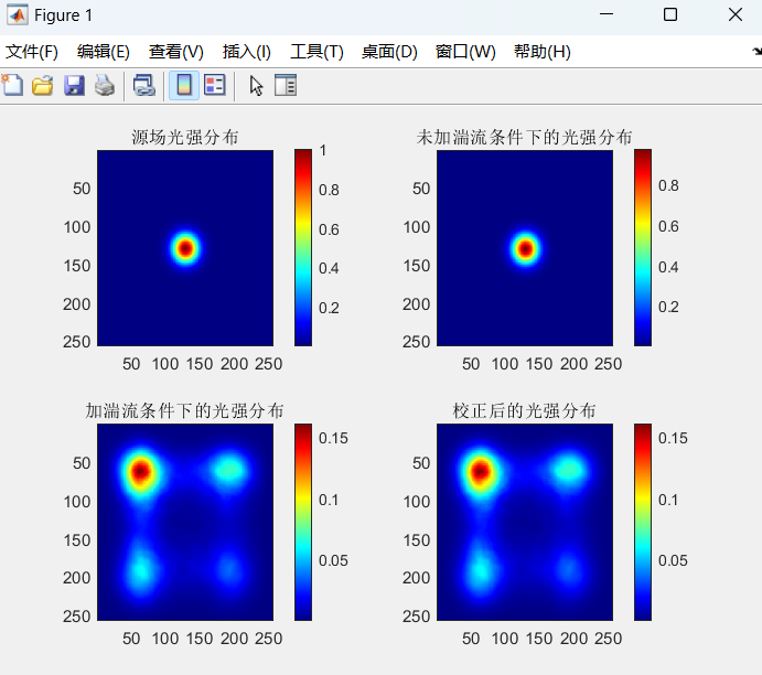
function visualize_results(I0, I1, I3, corrected_I, phase3,phase_reconstruction, phase_corrected, strehl_ratio, rmse)
figure(1);
% 显示未加湍流条件下的光强分布
subplot(2,2,1);
imagesc(I0);
title('源场光强分布');
colorbar;
colormap("jet");
% 显示未加湍流条件下的光强分布
subplot(2,2,2);
imagesc(I1);
title('未加湍流条件下的光强分布');
colorbar;
colormap("jet");
% 显示加湍流条件下的光强分布
subplot(2,2,3);
imagesc(I3);
title('加湍流条件下的光强分布');
colorbar;
colormap("jet");
% 显示校正后的光强分布
subplot(2,2,4);
imagesc(corrected_I);
title('校正后的光强分布');
colorbar;
colormap("jet")
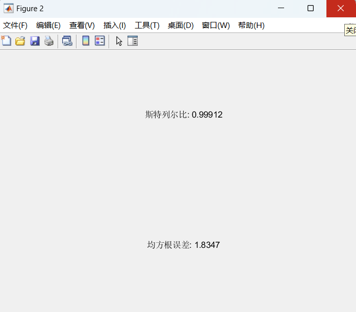
% 创建一个新的图用于显示斯特列尔比和均方根误差
figure(2);
% 显示斯特列尔比和均方根误差
text(0.5, 0.8, ['斯特列尔比: ', num2str(strehl_ratio)], 'HorizontalAlignment', 'center');
text(0.5, 0.2, ['均方根误差: ', num2str(rmse)], 'HorizontalAlignment', 'center');
axis off;
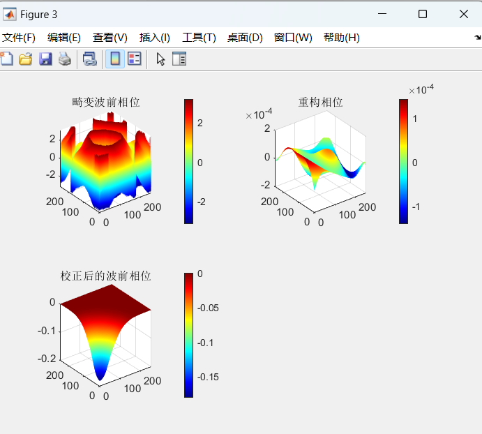
% 创建一个新的图用于显示波前相位分布
figure(3);
subplot(2,2,1);
surf(phase3);
title('畸变波前相位');
colorbar;
shading interp;
axis on;
axis square; % 输出正方形图像
subplot(2,2,2);
surf(phase_reconstruction);
title('重构相位');
colorbar;
shading interp;
axis on;
axis square; % 输出正方形图像
subplot(2,2,3);
surf(phase_corrected);
title('校正后的波前相位');
colorbar;
shading interp;
axis on;
axis square; % 输出正方形图像
end
```


