如何使用Python用辛普森方法确定一个函数在区间[a, b]上的积分的近似值

Question

要求将代码的“-----”部分补充完整，救救孩子的作业吧啊啊啊啊
以下为代码

import numpy as np
import matplotlib.pyplot as plt

#####################################################

FUNCTIONS

#####################################################
def SimpsonMethodValues(fvalues, a, b):
""" Simpson method for determining an approximation of
the integral of a function over the interval [a, b]
The function is known by its sampling "fvalues"
Input : fvalues = sampling of the function to be integrated (array)
: a,b = bounds of the interval
Output : S = Simpson approximation of the integral
"""
N = len(fvalues)
h = 2 * (b-a) / (N-1)
# partial sum S1
S1 = -----
S1 = S1 / 3.
# partial sum S2
S2 = -----
S2 = 2*S2 / 3.
# sum S
S = -----
S = S + S1 + S2
S *= h
return S

functions to be approximated :

def g0(x):
return np.ceil(x) # on ]-1,1]
def g1(x):
return x
def g2(x):
return x**2
def g3(x):
return np.abs(x)
def g4(x):
return np.sqrt(x)

#####################################################

MAIN

#####################################################
plt.cla()
plt.grid()

eps = 1e-10

Choice of a function :

f = g0; a = -1+eps; b = 1;
#f = g1; a = 0; b = 1;
#f = g2; a = -1; b = 1;
#f = g3; a = -1; b = 1;
#f = g4; a = 0; b = 1;

Period and pulsation

T = b-a;
w = 2*np.pi / T

Plot of the function to be approximated :

n = 8 # ==> 2^n+1 evaluation points (odd number of points)
t = np.linspace(a,b,2**n + 1) # for graph plotting
ft = f(t)
plt.plot(t-T,ft,'r')
plt.plot(t, ft,'r')
plt.plot(t+T,ft,'r')

N = 7

Fourier coefficients an and bn :

an = np.zeros(N+1)
bn = np.zeros(N+1)
an[0] = SimpsonMethodValues(ft, a, b) / T
for k in range(1,N+1):
-----
-----
-----
-----

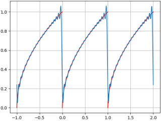
Fourier series at order N (over 3 periods)

tt = np.linspace(a-T,b+T,500)
ff = np.ones(np.size(tt))
ff = an[0] * ff
for k in range(1,N+1):
-----

plt.plot(tt,ff)

Answer 1

这道题是求给定函数的 傅里叶级数，其中采用 复化辛普森数值积分公式 计算傅里叶系数。下面索性倒着往前解答。

---

傅里叶级数

记不住傅里叶级数也没关系，随手搜一下：

（1）式对应最后一空，只不过这题只需取前 N 项

# Fourier series at order N (over 3 periods)
tt = np.linspace(a-T,b+T,500)
ff = np.ones(np.size(tt))
ff = an[0] * ff
for k in range(1,N+1):
    ff += an[k]*np.cos(k*w*tt) + bn[k]*np.sin(k*w*tt)   # <- 填空

继续往前，我们需要求解傅里叶系数 an 和 bn

以 an （系数数组的第 n 项）为例，它是一个积分式，被积函数 f(t) * cos(nwt)，积分区间 [a, b]。结合题意，采用辛普森方法进行数值积分，也就是前面定义的 SimpsonMethodValues()函数。

# Fourier coefficients an and bn :
an = np.zeros(N+1)
bn = np.zeros(N+1)
an[0] = SimpsonMethodValues(ft, a, b) / T
for k in range(1,N+1):
    ft_cos = ft * np.cos(k*w*t)    # <- 填空
    ft_sin = ft * np.sin(k*w*t)      # <- 填空
    an[k] = 2/T * SimpsonMethodValues(ft_cos, a, b)  # <- 填空
    bn[k] = 2/T * SimpsonMethodValues(ft_sin, a, b)   # <- 填空

复化辛普森数值积分公式

自然地，来到了辛普森数值积分函数的实现部分。辛普森方法是一种机械求积方式，通过复化（细分）积分区间的方式提升精度，具体参考百度百科的描述：

根据不同的表述方式，上图表达式稍微有所差异，但含义完全一致。注意这里采用的表述方式是：分为 2n 个子区间。于是，参数 fvalues 表示这 2n 个子区间的共计 2n+1 个端点，也就是 N = 2n+1 = len(fvalues)，即 n = (N-1)/2，进而 h = (b-a)/h = 2(b-a)/(N-1)。

结合已知的代码和上图，表达式右侧归纳为三部分：

• S： 两个端点对应的函数值
• S1：端点除外的所有偶数编号子节点对应函数值
• S2：端点除外的所有奇数编号子节点对应函数值

借助 Python 列表的切片表达式，很容易写出留空的部分：

def SimpsonMethodValues(fvalues, a, b):
    """ Simpson method for determining an approximation of
    the integral of a function over the interval [a, b]
    The function is known by its sampling "fvalues"
    Input : fvalues = sampling of the function to be integrated (array)
    : a,b = bounds of the interval
    Output : S = Simpson approximation of the integral
    """
    N = len(fvalues)
    h = 2 * (b-a) / (N-1)
    # partial sum S1
    S1 = np.sum(fvalues[2:N-2:2])    # <- 填空
    S1 = S1 / 3.
    # partial sum S2
    S2 = np.sum(fvalues[1:N-1:2])     # <- 填空
    S2 = 2*S2 / 3.
    # sum S
    S = (fvalues[0] + fvalues[-1]) / 6   # <- 填空
    S = S + S1 + S2
    S *= h
    return S

结果

填完空了，顺便跑一下结果吧。整个流程大意是用 N=7 阶傅里叶级数来近似原函数，然后在3个周期内画出对比图像。对了，最后加一个 plt.show()才能显示结果。以最后一个，[0, 1] 区间的平方根函数 f = √ x 为例：

• 红线为原函数
• 蓝线为傅里叶级数近似曲线