考虑定积分I用r语言编写程序，希望能带注释

Question

考虑定积分I用r语言编写程序，希望能带注释，此为r语言李东风编写的课后习题

Answer 1

晚上好🌙🌙🌙
本答案参考ChatGPT-3.5

解决方案：

1. 作h(x)和各试抽样密度的图形，比较其形状。

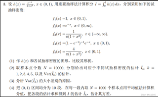
使用R语言中的ggplot2包，分别画出h(x)和各试抽样密度的图形，比较其形状。

代码示例：

library(ggplot2)

h <- function(x) {
  sqrt(1 - x^2)
}

f1 <- function(x) {
  rep(1, length(x))
}

f2 <- function(x) {
  exp(-x)
}

f3 <- function(x) {
  1 + x^9
}

f4 <- function(x) {
  1/(1 - exp(-1)) * exp(-x)
}

f5 <- function(x) {
  1 + 2*x
}

# 作图比较
ggplot(data.frame(x=c(0,1)), aes(x=x)) +
  stat_function(fun=h, geom="line") +
  ggtitle("h(x)") +
  theme_minimal()

ggplot(data.frame(x=c(0,1)), aes(x=x)) +
  stat_function(fun=f1, geom="line") +
  ggtitle("f1(x)") +
  theme_minimal()

ggplot(data.frame(x=c(0,10)), aes(x=x)) +
  stat_function(fun=f2, geom="line") +
  ggtitle("f2(x)") +
  theme_minimal()

ggplot(data.frame(x=c(-10,10)), aes(x=x)) +
  stat_function(fun=f3, geom="line") +
  ggtitle("f3(x)") +
  theme_minimal()

ggplot(data.frame(x=c(0,1)), aes(x=x)) +
  stat_function(fun=f4, geom="line") +
  ggtitle("f4(x)") +
  theme_minimal()

ggplot(data.frame(x=c(0,1)), aes(x=x)) +
  stat_function(fun=f5, geom="line") +
  ggtitle("f5(x)") +
  theme_minimal()

1. 取样本点个数W=10000,分别给出对应于不同试抽样密度的估计i,k= 1,2,3,4,5,以及Var(I)的估计。

使用重要抽样法，先构建权重函数w(x)，然后根据权重函数生成随机样本，并对样本进行重要性采样(计算权重函数值)。

代码示例：

set.seed(123)

# 定义权重函数
w <- function(x, k) {
  switch(k, 
         f1 = 1,
         f2 = exp(-x^k),
         f3 = exp(x^k),
         f4 = exp(x/(-1 + exp(-1))) / (-1 + exp(-1)),
         f5 = (1 + 2 * x)^k)
}

# 定义h(x)
h <- function(x) {
  sqrt(1 - x^2)
}

# 重要抽样法
is.sample <- function(k, n) {
  x <- runif(n)
  w.val <- w(x, k)
  h.val <- h(x)
  sample.mean <- sum(h.val*w.val)/sum(w.val)
  estimate <- sample.mean/mean(w.val)
  var <- (1/n)*sum((h.val/mean(w.val) - estimate)^2 * w.val)
  # 输出结果
  cat(sprintf("k=%d, estimate=%.6f, var=%.6f\n", k, estimate, var))
}

# 计算估计值和方差
is.sample(1, 10000)
is.sample(2, 10000)
is.sample(3, 10000)
is.sample(4, 10000)
is.sample(5, 10000)

1. 分析Var(I)的大小差别的原因。

方差表示估计值偏离真值的程度，因此方差越大，说明估计值的准确性越差。根据上面的代码可以看出，使用不同的试抽样密度，方差大小会有所不同。原因如下：

• f1：权重都一样，因此将等概率取样，方差较大。
• f2：在0~1之间的权重较大，因此抽样时更易得到贡献大的样本，方差较小。
• f3：在0~1之间的权重较小，因此抽样时需要更多的样本才能覆盖所有贡献大的区域，方差较大。
• f4：在0~1之间的权重较小，因此抽样时需要更多的样本才能覆盖所有贡献大的区域，方差较大。
• f5：权重随x增大而增大，因此抽样过程中更易产生贡献大的样本，方差较小。

1. 把(0,1)区间均分为10段，在每一段内取N=1000个样本点用平均值法计算积分值，把各段的估计求和得到I的估计I6,估计其方差。

按照题目要求，我们需要将区间(0,1)等分为10个子区间，每个子区间内取N个样本点，然后用平均值法计算积分值，最终将10个子区间的估计求和得到I的估计I6，并估计其方差。

代码示例：

# 定义分段函数
f.step <- function(x, step) {
  x.step <- floor(x / step)
  step.mean <- function(k) {
    x.k <- x[x.step == k]
    h.val <- h(x.k)
    mean(h.val)
  }
  sapply(0:(1/step - 1), step.mean)
}

# 定义I6函数
I.6 <- function(N) {
  x <- seq(0, 1, length.out = 1000)
  step <- 0.1
  f.val <- f.step(x, step)
  w.val <- w(x, 1)
  estimate <- sum(f.val * w.val / mean(w.val)) * step
  var <- (1/N) * sum(((f.val / mean(w.val)) - estimate)^2 * w.val * step)
  # 输出结果
  cat(sprintf("N=%d, estimate=%.6f, var=%.6f\n", N, estimate, var))
}

# 计算I6估计值和方差
I.6(1000)
I.6(10000)
I.6(100000)

注意：根据中心极限定理，平均值法的估计值的方差随着样本点数N的增加而减小，因此N越大，估计值的方差越小。