

多个样本 array list 怎么进行one-hot编码呢?
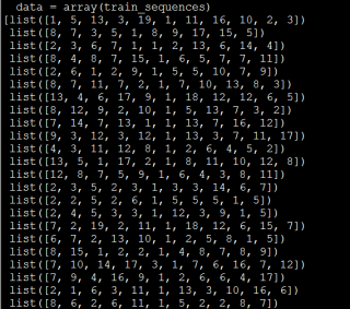
进行手动编码时报错


多个样本 array list 怎么进行one-hot编码呢?
进行手动编码时报错
 分享
分享 分享
分享  关注
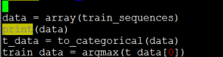
关注你之前的Tokenizer 以及 text_to_sequence 可能有问题
整完之后数据每行字母数都不一样了。

我自己尝试写了下字母转数字、然后array list转one-hot 编码方法

# print(keras._version_)
# print(tensorflow._version_)
# from tensorflow import keras
# from keras import backend as K#Keras 可以基于两个Backend,一个是 Theano,一个是 Tensorflow
import matplotlib.pyplot as plt  # 图形显示
import numpy as np
import pandas as pd  # pd.read_excel()方法读取excel文件
import tensorflow as tf
from sklearn import metrics
from sklearn.metrics import matthews_corrcoef  # 模型质量评价指数
from sklearn.model_selection import train_test_split  # 分割数据模块
from tensorflow.keras import layers
from tensorflow.keras.callbacks import EarlyStopping  # 早停,防止过拟合
from tensorflow.keras.callbacks import ModelCheckpoint  # 该回调函数将在每个epoch后保存模型到filepath
from tensorflow.keras.utils import to_categorical  # to_categorical就是将类别向量转换为二进制(只有0和1)的矩阵类型表示。其表现为将原有的类别向量转换为独热编码的形式。

# 预处理数据【找到所有的字母类型并对应0~ len(字母数)-1,然后进行转换】
# 按照此关系对应:{'A': 0, 'C': 1, 'D': 2, 'E': 3, 'F': 4, 'G': 5, 'H': 6, 'I': 7, 'K': 8, 'L': 9, 'M': 10, 'N': 11, 'P': 12, 'Q': 13, 'R': 14, 'S': 15, 'T': 16, 'V': 17, 'W': 18, 'Y': 19}
# 字母转数字  如 Y G Q E M Y V F R S E  转成 [19, 5, 13, 3, 10, 19, 17, 4, 14, 15, 3]
# 并转换为one-hot编码 (828,11) 转成 (828,11,20)
# 如     [[0. 0. 0. 0. 0. 0. 0. 0. 0. 0. 0. 0. 0. 0. 0. 0. 0. 0. 0. 1.]  第一行代表的Y值
#         [0. 0. 0. 0. 0. 1. 0. 0. 0. 0. 0. 0. 0. 0. 0. 0. 0. 0. 0. 0.]
#         [0. 0. 0. 0. 0. 0. 0. 0. 0. 0. 0. 0. 0. 1. 0. 0. 0. 0. 0. 0.]
#         [0. 0. 0. 1. 0. 0. 0. 0. 0. 0. 0. 0. 0. 0. 0. 0. 0. 0. 0. 0.]
#         [0. 0. 0. 0. 0. 0. 0. 0. 0. 0. 1. 0. 0. 0. 0. 0. 0. 0. 0. 0.]
#         [0. 0. 0. 0. 0. 0. 0. 0. 0. 0. 0. 0. 0. 0. 0. 0. 0. 0. 0. 1.]
#         [0. 0. 0. 0. 0. 0. 0. 0. 0. 0. 0. 0. 0. 0. 0. 0. 0. 1. 0. 0.]
#         [0. 0. 0. 0. 1. 0. 0. 0. 0. 0. 0. 0. 0. 0. 0. 0. 0. 0. 0. 0.]
#         [0. 0. 0. 0. 0. 0. 0. 0. 0. 0. 0. 0. 0. 0. 1. 0. 0. 0. 0. 0.]
#         [0. 0. 0. 0. 0. 0. 0. 0. 0. 0. 0. 0. 0. 0. 0. 1. 0. 0. 0. 0.]
#         [0. 0. 0. 1. 0. 0. 0. 0. 0. 0. 0. 0. 0. 0. 0. 0. 0. 0. 0. 0.]]
def preprocess_test_data(df_train):
    # 转换pd dataframe为 numpy,并获取x值
    np_df_train = np.array(df_train['文本'])
    print('origin: ', np_df_train[0])

    # 找到所有字母的分类及从0开始对应的字母标签值
    # {'A': 0, 'C': 1, 'D': 2, 'E': 3, 'F': 4, 'G': 5, 'H': 6, 'I': 7, 'K': 8, 'L': 9, 'M': 10, 'N': 11, 'P': 12, 'Q': 13, 'R': 14, 'S': 15, 'T': 16, 'V': 17, 'W': 18, 'Y': 19}
    # 注意 如果按照 A: 0  B:1 则转换的时候需要 A~Y 转成 24个字符表示,但此处需要表示为20个字符
    # 所以需要计算一个差值
    data_labels = sorted(
        set(np.array(sum([[j for j in list(str(i).replace(" ", ''))] for i in np_df_train], [])).flatten()))
    dict_lables = {}
    dict_labels_subtract = {}
    for index, j in enumerate(data_labels):
        dict_lables[j] = index
        dict_labels_subtract[j] = ord(j) - ord('A') - index
    print('data_labels: ', data_labels)
    print('dict_labels: ', dict_lables)
    print('dict_labels_subtract: ', dict_labels_subtract, len(dict_labels_subtract.keys()))

    # x = [[ord(j) - ord('A') for j in list(str(i).replace(" ", ''))] for i in np_df_train]
    # 转换每一个字母为 数字,按照A对应0  C对应1  D对应2 E对应3 Y对应19
    x = [[ord(j) - ord('A') - dict_labels_subtract[j] for j in list(str(i).replace(" ", ''))] for i in np_df_train]
    print('x[0]: ', x[0], type(x))

    # list转array
    labels = np.array(x)
    # 记录下数据原始的维度,方便进行one-hot编码后转回去
    labels_width, labels_height = labels.shape
    print('labels shape: ', labels.shape)
    set_n = sorted(set(labels.flatten()))
    print('sorted set_n: ', sorted(set_n), len(set_n), min(set_n), max(set_n))

    # 进行one-hot编码
    res = np.eye(len(set_n))[labels.flatten()]
    print("labels转成one-hot形式的结果:\n", res[0], "\n")
    print("labels转化成one-hot后的大小:", res.shape)

    # 成功实现one-hot编码 (828, 11)  -->  (828, 11, 20)
    train_data = res.reshape(labels_width, labels_height, len(set_n))
    print('转回原始数据的形式:', train_data[0], train_data.shape)
    return train_data

df_train = pd.read_excel(r'datas/yptrain.xlsx', sheet_name='训练集')
df_test = pd.read_excel(r'datas/yptest.xlsx', sheet_name='测试集')

# -----------------------------------------------------------------------------------------------------------------------------------------------------
# Y值的处理
lables_list = df_train['标签'].unique().tolist()  # unique():返回参数数组中所有不同的值,并按照从小到大排序,tolist()将数组或者矩阵转换成列表
dig_lables = dict(enumerate(lables_list))  # enumerate():列举,枚举,对一个列表,既要遍历索引又要遍历元素;dict:把enumerate()遍历到的转化为字典形式
# -----------------------------------------------------------------------------------------------------------------------------------------------------
# dict.items()列表返回可遍历的(键, 值) 元组数组.
# for dig, lable in dig_lables.items()就是遍历dig_lables里面的键(dig)和值(lable),
# dict((lable,dig) for dig, lable就是遍历dig和lable,让dig作为lable,lable作为dig
lable_dig = dict((lable, dig) for dig, lable in dig_lables.items())
df_train['标签_数字'] = df_train['标签'].apply(lambda lable: lable_dig[lable])  # 得到标签(lable)数字0和1
num_classes = len(dig_lables)  # dig_lables的长度即为num_classes
# 类别向量:df_train['标签_数字'],类别个数:num_classes,转换后的二进制矩阵:train_lables
train_lables = to_categorical(df_train['标签_数字'], num_classes=num_classes)  # to_categorical就是将类别向量转换为二进制(只有0和1)的矩阵类型表示。

# 预处理数据【找到所有的字母类型并对应0~ len(字母数)-1,然后进行转换】
# 按照此关系对应:{'A': 0, 'C': 1, 'D': 2, 'E': 3, 'F': 4, 'G': 5, 'H': 6, 'I': 7, 'K': 8, 'L': 9, 'M': 10, 'N': 11, 'P': 12, 'Q': 13, 'R': 14, 'S': 15, 'T': 16, 'V': 17, 'W': 18, 'Y': 19}
# 字母转数字  如 Y G Q E M Y V F R S E  转成 [19, 5, 13, 3, 10, 19, 17, 4, 14, 15, 3]
# 并转换为one-hot编码 (828,11) 转成 (828,11,20)
# 如     [[0. 0. 0. 0. 0. 0. 0. 0. 0. 0. 0. 0. 0. 0. 0. 0. 0. 0. 0. 1.]  第一行代表的Y值
#         [0. 0. 0. 0. 0. 1. 0. 0. 0. 0. 0. 0. 0. 0. 0. 0. 0. 0. 0. 0.]
#         [0. 0. 0. 0. 0. 0. 0. 0. 0. 0. 0. 0. 0. 1. 0. 0. 0. 0. 0. 0.]
#         [0. 0. 0. 1. 0. 0. 0. 0. 0. 0. 0. 0. 0. 0. 0. 0. 0. 0. 0. 0.]
#         [0. 0. 0. 0. 0. 0. 0. 0. 0. 0. 1. 0. 0. 0. 0. 0. 0. 0. 0. 0.]
#         [0. 0. 0. 0. 0. 0. 0. 0. 0. 0. 0. 0. 0. 0. 0. 0. 0. 0. 0. 1.]
#         [0. 0. 0. 0. 0. 0. 0. 0. 0. 0. 0. 0. 0. 0. 0. 0. 0. 1. 0. 0.]
#         [0. 0. 0. 0. 1. 0. 0. 0. 0. 0. 0. 0. 0. 0. 0. 0. 0. 0. 0. 0.]
#         [0. 0. 0. 0. 0. 0. 0. 0. 0. 0. 0. 0. 0. 0. 1. 0. 0. 0. 0. 0.]
#         [0. 0. 0. 0. 0. 0. 0. 0. 0. 0. 0. 0. 0. 0. 0. 1. 0. 0. 0. 0.]
#         [0. 0. 0. 1. 0. 0. 0. 0. 0. 0. 0. 0. 0. 0. 0. 0. 0. 0. 0. 0.]]
train_data = preprocess_test_data(df_train)
print('Shape of data train:', train_data.shape)

# 划分训练集和验证集
# n_splits:折叠次数,默认为3,至少为2。shuffle:是否在每次分割之前打乱顺序。
# random_state:随机种子,在shuffle==True时使用,默认使用np.random。
'''skf = StratifiedKFold(n_splits=5, random_state=None, shuffle=True)
skf.get_n_splits(train_data, df_train['标签'])#给出K折的折数,输出为5
#print(skf)#输出为:StratifiedKFold(n_splits=5,random_state=None, shuffle=True)
for train_index, val_index in skf.split(train_data, df_train['标签']):
#    print("TRAIN:", train_index, "TEST:", val_index)#得到验证集和训练集的索引(index)
#    print(len(train_index),len(val_index))
    DATA_train, x_val = train_data[train_index], train_data[val_index]#训练集和验证集的data数据
    LABLES_train, y_val = df_train['标签'][train_index], df_train['标签'][val_index] # 练集和验证集的lables'''
# 随机种子
seed = 7
np.random.seed(seed)
DATA_train, x_val, LABLES_train, y_val = train_test_split(train_data, df_train['标签_数字'], test_size=0.2, random_state=0,
                                                          shuffle=True)
model = tf.keras.Sequential()
print('train_data: ', DATA_train.shape, LABLES_train.shape)
print('test_data: ', x_val.shape, y_val.shape)
# model.add(layers.Embedding(input_dim=vocab_size, output_dim=128, mask_zero=True, embeddings_initializer='uniform'))
# model.add(layers.BatchNormalization())model.add(layers.SpatialDropout1D(0.4))
# model.add(layers.GRU(128, return_sequences=False, dropout=0.2, recurrent_dropout=0.2))

model.add(layers.LSTM(128, return_sequences=False, dropout=0.2, recurrent_dropout=0.2, input_shape=(11, 20)))
model.add(layers.BatchNormalization())
model.add(layers.Dense(256, activation='relu', kernel_initializer='glorot_uniform'))
model.add(layers.BatchNormalization())
model.add(layers.Dense(1024, activation='relu', kernel_initializer='glorot_uniform'))
model.add(layers.BatchNormalization())
model.add(layers.Dense(1024, activation='relu', kernel_initializer='glorot_uniform'))
model.add(layers.BatchNormalization())
model.add(layers.Dense(256, activation='relu', kernel_initializer='glorot_uniform'))
# model.add(layers.BatchNormalization())
model.add(layers.Dense(256, activation='relu', kernel_initializer='glorot_uniform'))
model.add(layers.BatchNormalization())
model.add(layers.Dense(2, activation='softmax'))
model.summary()
opt = tf.keras.optimizers.RMSprop(learning_rate=0.001, rho=0.9)
model.compile(optimizer=opt, loss='sparse_categorical_crossentropy', metrics=['accuracy'])
# -----------------------------------------------------------------------------------------------------------------------------------------------------
# early_stopping
# This callback will interrupt training when we have stopped improving
early_stopping = EarlyStopping(
    # This callback will monitor the validation accuracy of the model
    monitor='val_accuracy',  # 需要监视的量,val_loss,val_accuracy
    # Training will be interrupted when the accuracy
    # has stopped improving for *more* than 1 epochs (i.e. 2 epochs)
    patience=10,  # 当early stop被激活(如发现loss相比上一个epoch训练没有下降),则经过patience个epoch后停止训练
    verbose=1,  # 信息展示模式
    mode='max')  # 'auto','min','max'之一,在min模式训练,如果检测值停止下降则终止训练。在max模式下,当检测值不再上升的时候则停止训练。
# -----------------------------------------------------------------------------------------------------------------------------------------------------
# 模型保存
# This callback will save the current weights after every epoch
Checkpoint = ModelCheckpoint(
    'datas' + '/model-{epoch:02d}.hdf5',  # 字符串,保存模型的路径。

    monitor='val_accuracy',  # 被监测的数据。val_accuracy或这val_loss
    verbose=1,  # 详细信息模式,0 或者 1 。0为不打印输出信息,1打印
    save_best_only=True,  # 如果 save_best_only=True, 将只保存在验证集上性能最好的模型
    save_weights_only=False,
    # 如果 True,那么只有模型的权重会被保存 (model.save_weights(filepath)), 否则的话,整个模型会被保存 (model.save(filepath))。
    mode='auto',
    # {auto, min, max} 的其中之一。 如果 save_best_only=True,那么是否覆盖保存文件的决定就取决于被监测数据的最大或者最小值。 对于 val_accuracy,模式就会是 max,而对于 val_loss,模式就需要是 min,等等。 在 auto 模式中,方向会自动从被监测的数据的名字中判断出来。
    period=50)  # 每个检查点之间的间隔(训练轮数)。
# -----------------------------------------------------------------------------------------------------------------------------------------------------
cw = {0: 0.67, 1: 1.93}
# cw = {0:1, 1:7.}
# cw = {0:0.7, 1:1.73}#A
# cw = {0:0.63,1: 2.47}#B
# cw = {0:0.83, 1:1.26}#c

# print('Resampled dataset shape %s' % Counter(y_train_res))
history = model.fit(DATA_train, LABLES_train, batch_size=128, shuffle=True, epochs=2, validation_data=(x_val, y_val),
                    callbacks=[early_stopping, Checkpoint], class_weight=cw)
# history = parallel_model.fit(DATA_train,LABLES_train,batch_size=128,shuffle=True,epochs=3,validation_data=(x_val,y_val),callbacks=[early_stopping,Checkpoint])
# history = model.fit(DATA_train,LABLES_train,batch_size=128,steps_per_epoch =156844,shuffle=True,epochs=3,validation_data=(x_val,y_val),callbacks=[early_stopping,Checkpoint],class_weight=cw)
# history = model.fit(DATA_train,LABLES_train,batch_size=128,shuffle=True,epochs=200,validation_data=(x_val,y_val),callbacks=[early_stopping,Checkpoint])
# Evaluating the model
# history = model.fit(DATA_train,LABLES_train,batch_size=128,shuffle=True,epochs=200,validation_data=(x_val,y_val),callbacks=[early_stopping,Checkpoint])

score = model.evaluate(DATA_train, LABLES_train, verbose=0)
print('train Loss:', score[0])
print('train Accuracy:', score[1])

# -----------------------------------------------------------------------------------------------------------------------------------------------------
predict_val = model.predict(DATA_train)
predict_val = predict_val.argmax(axis=1)
print('val-predict_val:', predict_val.shape)

# predict_classes = model.predict_classes(DATA_train)
# print('train-predict_classes:',predict_classes)
# -----------------------------------------------------------------------------------------------------------------------------------------------------
tn, fp, fn, tp = metrics.confusion_matrix(LABLES_train, predict_val).ravel()
spe = tn / (tn + fp)  # 特异性
print('train-spe:', spe)
# -----------------------------------------------------------------------------------------------------------------------------------------------------
# recall_score,召回率=提取出的正确信息条目数/样本中的信息条目数。也就是所有准确的条目有多少被检索出来了
# 也被称为查全率,在医学上常常被称作敏感度(Sensitive),召回率的定义是,在所有实际为正例的样本中,被预测为正例的样本比例,
# recall,正确预测为正的,占全部实际为正的比例,TP / (TP+FN)
sen = metrics.recall_score(LABLES_train, predict_val)  # 敏感度
print('train-sen:', sen)
# -----------------------------------------------------------------------------------------------------------------------------------------------------
# roc_auc_score,计算了ROC曲线下面的面积,它也被称为AUC或AUROC。通过计算下面的面积,曲线信息被归一化到1内。
auc1 = metrics.roc_auc_score(LABLES_train, predict_val)
print('train-auc:', auc1)
# -----------------------------------------------------------------------------------------------------------------------------------------------------
mcc = matthews_corrcoef(LABLES_train, predict_val)
print('train-mcc:', mcc)

F1 = metrics.f1_score(LABLES_train, predict_val)  # 敏感度
print('train-F:', F1)

print('训练集验证集完成======================================================')

# -----------------------------------------------------------------------------------------------------------------------------------------------------
# Evaluating the model
score = model.evaluate(x_val, y_val, verbose=0)
print('Val Loss:', score[0])
print('Val Accuracy:', score[1])

# -----------------------------------------------------------------------------------------------------------------------------------------------------
predict_val = model.predict(x_val)
# print('val-predict_val:',predict_val)
predict_val = predict_val.argmax(axis=1)
print('val-predict_val:', predict_val.shape)
# predict_classes = model.predict_classes(x_val)
# print('val-predict_classes:', predict_classes)
# -----------------------------------------------------------------------------------------------------------------------------------------------------
tn, fp, fn, tp = metrics.confusion_matrix(y_val, predict_val).ravel()
spe = tn / (tn + fp)  # 特异性
print('val-spe:', spe)
# -----------------------------------------------------------------------------------------------------------------------------------------------------
# recall_score,召回率=提取出的正确信息条目数/样本中的信息条目数。也就是所有准确的条目有多少被检索出来了
# 也被称为查全率,在医学上常常被称作敏感度(Sensitive),召回率的定义是,在所有实际为正例的样本中,被预测为正例的样本比例,
# recall,正确预测为正的,占全部实际为正的比例,TP / (TP+FN)
sen = metrics.recall_score(y_val, predict_val)  # 敏感度
print('val-sen:', sen)
# -----------------------------------------------------------------------------------------------------------------------------------------------------
# roc_auc_score,计算了ROC曲线下面的面积,它也被称为AUC或AUROC。通过计算下面的面积,曲线信息被归一化到1内。
auc2 = metrics.roc_auc_score(y_val, predict_val)
print('val-auc:', auc2)

# -----------------------------------------------------------------------------------------------------------------------------------------------------
mcc = matthews_corrcoef(y_val, predict_val)
print('val-mcc:', mcc)

F = metrics.f1_score(y_val, predict_val)  # 敏感度
print('val-F:', F)

print('训练集验证集完成======================================================')
# -----------------------------------------------------------------------------------------------------------------------------------------------------
# 保存模型
model.save('datas/GRU_.h5')
# 加载模型
model = tf.keras.models.load_model('datas/GRU_.h5')
model.summary()

test_data = preprocess_test_data(df_test)
print("Shape of data test: ",test_data.shape)
pred_ = model.predict(test_data)
print('pred_: ', pred_)
pred_ = pred_.argmax(axis=1)

df_test['分类结果_预测'] = [dig_lables[dig] for dig in pred_]
print('test-accuracy_score:', metrics.accuracy_score(df_test['标签'], df_test['分类结果_预测']))
# -----------------------------------------------------------------------------------------------------------------------------------------------------
# 测试集结果度量
# Confusion_matrix
tn, fp, fn, tp = metrics.confusion_matrix(df_test['标签'], df_test['分类结果_预测']).ravel()
spe = tn / (tn + fp)  # 特异性
print('test-spe:', spe)
# -----------------------------------------------------------------------------------------------------------------------------------------------------
# recall_score,召回率=提取出的正确信息条目数/样本中的信息条目数。也就是所有准确的条目有多少被检索出来了
# 也被称为查全率,在医学上常常被称作敏感度(Sensitive),召回率的定义是,在所有实际为正例的样本中,被预测为正例的样本比例,
# recall,正确预测为正的,占全部实际为正的比例,TP / (TP+FN)
sen = metrics.recall_score(df_test['标签'], df_test['分类结果_预测'])  # 敏感度
print('test-sen:', sen)
# -----------------------------------------------------------------------------------------------------------------------------------------------------
# # roc_auc_score,计算了ROC曲线下面的面积,它也被称为AUC或AUROC。通过计算下面的面积,曲线信息被归一化到1内。
# y_pred = model.predict_proba(test_data)[:, 1]
# # print('y_pred',y_pred)
# fpr, tpr, thresholds = roc_curve(df_test['标签'], y_pred)
# print('auc1:', auc(fpr, tpr))

auc = metrics.roc_auc_score(df_test['标签'], df_test['分类结果_预测'])
print('test-auc:', auc)
# -----------------------------------------------------------------------------------------------------------------------------------------------------
mcc = matthews_corrcoef(df_test['标签'], df_test['分类结果_预测'])
print('test-mcc:', mcc)
# -----------------------------------------------------------------------------------------------------------------------------------------------------
# 精确率,precision,正确预测为正的,占全部预测为正的比例,TP / (TP+FP)
precision_recall_curve = metrics.precision_recall_curve(df_test['标签'], df_test['分类结果_预测'])
print('precision_recall_curve:', precision_recall_curve)

# F-Measure是Precision和Recall加权调和平均,当F1较高时则比较说明实验方法比较理想。
f1_score = metrics.f1_score(df_test['标签'], df_test['分类结果_预测'], labels=None, pos_label=1, average='micro',
                            sample_weight=None)
print('f1_score3:', f1_score)
# f1_score=metrics.f1_score(df_test['标签'],df_test['分类结果_预测'], labels=None, pos_label=1, average='weighted', sample_weight=None)
# print('f1_score4:',f1_score)

# from sklearn.metrics import balanced_accuracy_score
balanced_accuracy_score = metrics.balanced_accuracy_score(df_test['标签'], df_test['分类结果_预测'], sample_weight=None,
                                                          adjusted=False)
print('balanced_accuracy_score:', balanced_accuracy_score)

plt.figure(1)
print('训练集验证集图形')
epoch = np.arange(1, len(history.history['loss']) + 1, 1)  # 设置图形的x坐标值
font2 = {  # 'family' : 'Times New Roman',
    'size': 14, }
# plt.title('Loss')#图形的标题:Loss
plt.plot(epoch, history.history['loss'], label='Training set')  # 训练集的loss图形
plt.plot(epoch, history.history['val_loss'], label='Validation set')  # 验证集的loss图形
plt.xlabel("Epoch", font2)
plt.ylabel("Loss", font2)
plt.ylim((0.1, 0.8))  # 设置x坐标轴的范围
plt.legend(loc='best', frameon=False)  # 去掉图例边框
plt.legend(prop=font2)  # 主要的作用就是给图加上图例,plt.legend([x,y,z])里面的参数使用的是list的的形式将图表的的名称喂给这和函数。
# plt.show()  # 显示图形
plt.savefig('datas/GRU_01.png')

# -----------------------------------------------------------------------------------------------------------------------------------------------------
plt.figure(2)

print('model fit history: ', history.history)
epoch = np.arange(1, len(history.history['accuracy']) + 1, 1)  # 设置图形的x坐标值
font2 = {  # 'family' : 'Times New Roman',
    'size': 14, }
# plt.title('Accuracy')#图形的标题:Accuracy
plt.plot(epoch, history.history['accuracy'], label='Training set')  # 训练集的acc图形
plt.plot(epoch, history.history['val_accuracy'], label='Validation set')  # 验证集的loss图形:val_accuracy
plt.xlabel("Epoch", font2)
plt.ylabel("Accuracy", font2)
plt.ylim((0.5, 1))  # 设置x坐标轴的范围
plt.legend(loc='best', frameon=False)  # 去掉图例边框
plt.legend(prop=font2)  # 主要的作用就是给图加上图例,plt.legend([x,y,z])里面的参数使用的是list的的形式将图表的的名称喂给这和函数。
# plt.show()  # 显示图形
plt.savefig('datas/GRU_02.png')

plt.figure(3)
print('训练集验证集图形')
epoch = np.arange(1, len(history.history['loss']) + 1, 1)  # 设置图形的x坐标值
font2 = {  # 'family' : 'Times New Roman',
    'size': 14, }

# plt.title('Loss')#图形的标题:Loss
plt.plot(epoch, history.history['loss'], label='Training set')  # 训练集的loss图形
plt.plot(epoch, history.history['val_loss'], label='Validation set')  # 验证集的loss图形

plt.xlabel("Epoch", font2)
plt.ylabel("Loss", font2)
plt.ylim((0.2, 1))  # 设置x坐标轴的范围
plt.legend(loc='best', frameon=False)  # 去掉图例边框
plt.legend(prop=font2)  # 主要的作用就是给图加上图例,plt.legend([x,y,z])里面的参数使用的是list的的形式将图表的的名称喂给这和函数。
# plt.show()  # 显示图形
plt.savefig('datas/GRU_03.png')
 系统已结题
9月14日
系统已结题
9月14日 创建了问题
9月7日
创建了问题
9月7日